Day 12: A challenge to learn basics of Structural Equation Modeling (SEM) using lavaan and semPlot packages in R

 

During the next 12 days, I will learn and repeat the basics of structural equation modeling (SEM) using lavaan and semPlot packages in R.

You can search my lavaan posts by typing: #UsmanZafarParacha_lavaan , and semPlot posts by typing: #UsmanZafarParacha_semPlot

=============

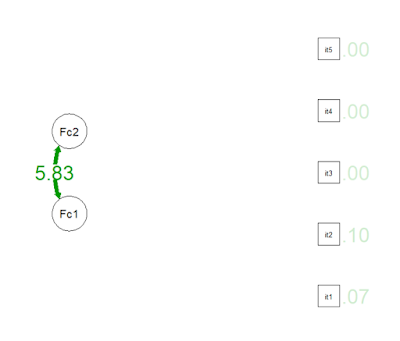
During this day, I learned and studied about Confirmatory Factor Analysis (CFA) while implementing a polychoric matrix and use the robust diagonally weighted least squares (RDWLS) method to evaluate the model fit using several fit indices such as RMSEA, CFI, TLI, SRMR, and chi-square/DF. This same thing can also be found in one of the research papers, such as that conducted Almeida et al. (2024).

Initially, I loaded the essential libraries and created supposed data using the following lines of codes:

 

library(lavaan)

library(semPlot)

library(psych)

 

set.seed(123)  # For reproducibility

n <- 200  # Number of participants

 

# Simulate ordinal data (Likert scale: 1 to 5)

item1 <- sample(1:5, n, replace = TRUE)

item2 <- sample(1:5, n, replace = TRUE)

item3 <- sample(1:5, n, replace = TRUE)

item4 <- sample(1:5, n, replace = TRUE)

item5 <- sample(1:5, n, replace = TRUE)

 

# Create a data frame

data <- data.frame(item1, item2, item3, item4, item5)

 

Then, using the psych package, the polychoric correlation matrix was determined:

 

polychoric_matrix <- polychoric(data)$rho

 

The CFA model was specified:

 

cfa_model <- '

  Factor1 =~ item1 + item2 + item3

  Factor2 =~ item4 + item5

'

 

fit <- cfa(cfa_model, sample.cov = polychoric_matrix, sample.nobs = n, estimator = "ML")

 

and the model fit was checked:

 

summary(fit, fit.measures = TRUE, standardized = TRUE)

 

Eventually, the CFA model was visualized:

 

semPaths(fit, what = "std", edge.label.cex = 1.2, layout = "tree", style = "lisrel", rotation = 2)

 

 

Sources:

Almeida, D. M., Santos-de-Araújo, A. D., Júnior, J. M. C. B., Cacere, M., Pontes-Silva, A., Costa, C. P., ... & Bassi-Dibai, D. (2024). The best internal structure of the Diabetes Quality of Life Measure (DQOL) in Brazilian patients. BMC Public Health, 24(1), 580.

ChatGPT

Day 11: A challenge to learn basics of Structural Equation Modeling (SEM) using lavaan and semPlot packages in R

 During the next 12 days, I will learn and repeat the basics of structural equation modeling (SEM) using lavaan and semPlot packages in R.

You can search my lavaan posts by typing: #UsmanZafarParacha_lavaan , and semPlot posts by typing: #UsmanZafarParacha_semPlot

=============

During this day, I loaded lavaan and semPlot, and defined the SEM model, as follows:

# Load the packages

library(lavaan)

library(semPlot)

 

# Define the SEM model

model <- '

  # Direct effect

  productivity ~ management + job_satisfaction + workplace

 

  # Indirect effect

  job_satisfaction ~ management

'

 

Then, a supposed data was developed, as follows:

# Simulate a dataset with the relevant variables

set.seed(123)  # For reproducibility

 

n <- 200  # Number of observations

 

# Simulate random variables for the model

management <- rnorm(n, mean = 5, sd = 2)  # Management style

job_satisfaction <- 0.5 * management + rnorm(n, mean = 0, sd = 1)  # Job satisfaction

workplace <- rnorm(n, mean = 4, sd = 1.5)  # Workplace environment

productivity <- 0.3 * management + 0.4 * job_satisfaction + 0.5 * workplace + rnorm(n, mean = 0, sd = 1)  # Productivity

 

# Combine into a data frame

data <- data.frame(management, job_satisfaction, workplace, productivity)

 

# Inspect the data

head(data)

 

Then, lavaan was used to fit the SEM model, as follows:

 

# Fit the model

fit <- sem(model, data = data)

 

# Display the summary of the SEM results

summary(fit, fit.measures = TRUE, standardized = TRUE, rsquare = TRUE)

 

Eventually, the model is visualized using the semPlot package, as follows:

# Visualize the SEM model

semPaths(fit, what = "std", layout = "tree", edge.label.cex = 1.2,

         style = "ram", nCharNodes = 0, curvePivot = TRUE)

 

Source:

ChatGPT

Day 10: A challenge to learn basics of Structural Equation Modeling (SEM) using lavaan and semPlot packages in R

 During the next 12 days, I will learn and repeat the basics of structural equation modeling (SEM) using lavaan and semPlot packages in R.

You can search my lavaan posts by typing: #UsmanZafarParacha_lavaan , and semPlot posts by typing: #UsmanZafarParacha_semPlot

=============

During this day, I loaded the essential libraries, and defined the SEM model using the following lines of codes:

 

# Load libraries

library(lavaan)

library(semPlot)

 

# Define the SEM model

model <- '

  # Direct effect of teacher experience on instructional methods

  InstructionalMethods ~ a * TeacherExperience

 

  # Direct effect of instructional methods on student performance

  StudentPerformance ~ b * InstructionalMethods

 

  # Direct effect of teacher experience on student performance

  StudentPerformance ~ c * TeacherExperience

 

  # Moderation: Classroom environment moderates the effect of instructional methods on student performance

  StudentPerformance ~ d * Interaction

 

  # Define indirect (mediation) effect

  indirect := a * b

 

  # Define total effect (direct + indirect effects)

  total := c + (a * b)

'

 

Then, a supposed data is generated using the following lines of codes:

 

# Generate sample data (if real data is not available)

set.seed(123)

n <- 300

data <- data.frame(

  TeacherExperience = rnorm(n, mean = 10, sd = 5),

  ClassroomEnvironment = rnorm(n, mean = 3, sd = 1),

  InstructionalMethods = rnorm(n, mean = 0, sd = 1),

  StudentPerformance = rnorm(n, mean = 75, sd = 10)

)

 

Then a relationship is created and interaction terms are established, as follows:

 

# Create relationships and interaction term

data$InstructionalMethods <- 0.5 * data$TeacherExperience + rnorm(n)

data$StudentPerformance <- 0.3 * data$TeacherExperience +

                           0.6 * data$InstructionalMethods +

                           0.4 * data$InstructionalMethods * data$ClassroomEnvironment +

                           rnorm(n)

data$Interaction <- data$InstructionalMethods * data$ClassroomEnvironment

 

Then we fit the model and visualized the SEM model using the following lines of codes:

 

# Fit the model

fit <- sem(model, data = data)

summary(fit, standardized = TRUE, fit.measures = TRUE)

 

# Visualize the SEM model

semPaths(fit,

         whatLabels = "std",

         layout = "tree",

         edge.color = "blue",

         sizeMan = 6,

         sizeLat = 8,

         fade = FALSE)

 

Source:

ChatGPT

Day 9: A challenge to learn basics of Structural Equation Modeling (SEM) using lavaan and semPlot packages in R

 

During the next 12 days, I will learn and repeat the basics of structural equation modeling (SEM) using lavaan and semPlot packages in R.

You can search my lavaan posts by typing: #UsmanZafarParacha_lavaan , and semPlot posts by typing: #UsmanZafarParacha_semPlot

=============

During this day, I loaded essential libraries, and defined the SEM model, using the following lines of codes:

# Load the libraries

library(lavaan)

library(semPlot)

 

# Define the SEM model

model <- '

  # Direct effects

  Housing_Demand ~ Economic_Conditions

  Property_Prices ~ Housing_Demand

 

  # Moderation (interaction term between Housing Demand and Interest Rates)

  Property_Prices ~ Housing_Demand * Interest_Rates

'

 

Then develop a supposed dataset using the following:

# Simulate data for the model

set.seed(123) # For reproducibility

N <- 300 # Sample size

 

Economic_Conditions <- rnorm(N, mean = 0, sd = 1)

Housing_Demand <- 0.6 * Economic_Conditions + rnorm(N, mean = 0, sd = 1)

Interest_Rates <- runif(N, min = 2, max = 5)  # Random interest rates between 2% and 5%

Property_Prices <- 0.8 * Housing_Demand + 0.4 * Housing_Demand * Interest_Rates + rnorm(N, mean = 0, sd = 1)

 

# Combine data into a dataframe

data <- data.frame(Economic_Conditions, Housing_Demand, Interest_Rates, Property_Prices)

 

Then I fit the SEM model using lavaan, as follows:

 

# Fit the SEM model

fit <- sem(model, data = data)

 

# Display the summary of the SEM model

summary(fit, fit.measures = TRUE, standardized = TRUE)

 

Eventually, the model is visualized using semPlot, as follows:

# Plot the SEM model

semPaths(fit, "std", whatLabels = "std", edge.label.cex = 1.2, layout = "tree",

         style = "lisrel", residuals = FALSE, intercepts = FALSE)

 

Source:
ChatGPT

Day 8: A challenge to learn basics of Structural Equation Modeling (SEM) using lavaan and semPlot packages in R

 

During the next 12 days, I will learn and repeat the basics of structural equation modeling (SEM) using lavaan and semPlot packages in R.

You can search my lavaan posts by typing: #UsmanZafarParacha_lavaan , and semPlot posts by typing: #UsmanZafarParacha_semPlot

=============

During this day, I loaded the essential libraries and prepared a data, using the following lines of codes:

 

# Load the required libraries

library(lavaan)

library(semPlot)

library(psych)

 

# Simulate data

set.seed(123)  # For reproducibility

n <- 300  # Number of samples

 

# Latent variables

Knowledge <- rnorm(n, mean = 0, sd = 1)

Attitudes <- 0.5 * Knowledge + rnorm(n, mean = 0, sd = 1)

Behavior <- 0.7 * Knowledge + 0.4 * Attitudes + rnorm(n, mean = 0, sd = 1)

 

# Observed indicators for each latent variable

Know1 <- 0.8 * Knowledge + rnorm(n, mean = 0, sd = 0.5)

Know2 <- 0.9 * Knowledge + rnorm(n, mean = 0, sd = 0.5)

Know3 <- 0.7 * Knowledge + rnorm(n, mean = 0, sd = 0.5)

 

Att1 <- 0.8 * Attitudes + rnorm(n, mean = 0, sd = 0.5)

Att2 <- 0.9 * Attitudes + rnorm(n, mean = 0, sd = 0.5)

Att3 <- 0.7 * Attitudes + rnorm(n, mean = 0, sd = 0.5)

 

Beh1 <- 0.8 * Behavior + rnorm(n, mean = 0, sd = 0.5)

Beh2 <- 0.9 * Behavior + rnorm(n, mean = 0, sd = 0.5)

Beh3 <- 0.7 * Behavior + rnorm(n, mean = 0, sd = 0.5)

 

# Create a data frame

data <- data.frame(Know1, Know2, Know3, Att1, Att2, Att3, Beh1, Beh2, Beh3)

 

The above code shows three observed variables for each latent factor. For example,

Knowledge: Know1, Know2, Know3

Attitudes: Att1, Att2, Att3

Behavior: Beh1, Beh2, Beh3

Then the SEM model is specified, using the following lines of codes:

 

# SEM model specification

model <- '

  # Measurement model

  Knowledge =~ Know1 + Know2 + Know3

  Attitudes =~ Att1 + Att2 + Att3

  Behavior  =~ Beh1 + Beh2 + Beh3

 

  # Structural model

  Attitudes ~ Knowledge

  Behavior  ~ Knowledge + Attitudes

'

The SEM model is fitted using lavaan, and visualized using the semPaths, as follows:

 

# Fit the SEM model

fit <- sem(model, data = data)

 

# Summarize the results

summary(fit, fit.measures = TRUE, standardized = TRUE)

 

# Plot the SEM path diagram

semPaths(fit, "std", layout = "tree", residuals = TRUE, nCharNodes = 7, edge.label.cex = 1.2)

 

Source:
ChatGPT

Day 7: A challenge to learn basics of Structural Equation Modeling (SEM) using lavaan and semPlot packages in R

During the next 12 days, I will learn and repeat the basics of structural equation modeling (SEM) using lavaan and semPlot packages in R.

You can search my lavaan posts by typing: #UsmanZafarParacha_lavaan , and semPlot posts by typing: #UsmanZafarParacha_semPlot

=============

During this day, I loaded essential libraries, including lavaan and semPlot, and then defined the SEM model, as follows:

 

library(lavaan)

library(semPlot)

 

# Define the SEM model

model <- '

  # Direct effects

  Z ~ b1*X + b2*Y

 

  # Indirect effects (X affects Z through Y)

  Y ~ a1*X

 

  # Calculate the indirect effect

  indirect := a1 * b2

 

  # Total effect of X on Z

  total := b1 + (a1 * b2)

'

 

These aspects can be explained as follows:

·        Z ~ b1X + b2Y: Disease risk (Z) is predicted by genetic predisposition (X) and environmental factors (Y).

·        Y ~ a1*X: Environmental factors (Y) are predicted by genetic predisposition (X).

·        indirect := a1 * b2: Defines the indirect effect of genetic predisposition (X) on disease risk (Z) through environmental factors (Y).

·        total := b1 + (a1 * b2): Defines the total effect of genetic predisposition (X) on disease risk (Z), which includes both the direct and indirect effects.

Then the supposed data is generated as follows:

# Set seed for reproducibility

set.seed(123)

 

# Simulate data with 300 observations

n <- 300

X <- rnorm(n, mean = 0, sd = 1)  # Genetic predisposition

Y <- 0.6 * X + rnorm(n, mean = 0, sd = 1)  # Environmental factors influenced by X

Z <- 0.5 * X + 0.7 * Y + rnorm(n, mean = 0, sd = 1)  # Disease risk influenced by X and Y

 

# Combine into a data frame

data <- data.frame(X = X, Y = Y, Z = Z)

 

Then, the SEM model is fitted using the following codes:

 

# Fit the SEM model to the data

fit <- sem(model, data = data)

 

# Summarize the model fit

summary(fit, fit.measures = TRUE, standardized = TRUE)

 

The model is visualized using the following lines of codes:

 

# Visualize the SEM model using semPlot

semPaths(fit, what = "std", layout = "tree", edge.label.cex = 1.2,

         nCharNodes = 6, edge.color = "blue", style = "lisrel")

Source:
ChatGPT

 

Day 5: A challenge to learn basics of Structural Equation Modeling (SEM) using lavaan and semPlot packages in R

During the next 12 days, I will learn and repeat the basics of structural equation modeling (SEM) using lavaan and semPlot packages in R.

You can search my lavaan posts by typing: #UsmanZafarParacha_lavaan , and semPlot posts by typing: #UsmanZafarParacha_semPlot

============

During this day, I loaded lavaan and semPlot packages. Then, defined the model using the following lines of codes:

 

 

# Define the SEM model

model <- '

  # Direct effects

  achievement ~ teaching_quality + peer_support + engagement

 

  # Indirect effects

  engagement ~ peer_support

 

  # Covariances (optional if you want to assess relationships between predictors)

  peer_support ~~ teaching_quality

'

 

Then, created a supposed data using the following lines of codes:

 

# Simulate data (for the sake of demonstration)

set.seed(123)

n <- 200

peer_support <- rnorm(n, mean = 5, sd = 2)

teaching_quality <- rnorm(n, mean = 6, sd = 1.5)

engagement <- 0.5 * peer_support + rnorm(n, mean = 3, sd = 1)

achievement <- 0.6 * teaching_quality + 0.3 * peer_support + 0.4 * engagement + rnorm(n)

 

data <- data.frame(peer_support, teaching_quality, engagement, achievement)

 

Then, I fit the SEM model to the data:

 

# Fit the model

fit <- sem(model, data = data)

# Get a summary of the model

summary(fit, fit.measures = TRUE, standardized = TRUE)

 

Then, the SEM model is visualized using the following lines of codes:

# Plot the SEM model

semPaths(fit, what = "std", layout = "tree", edge.label.cex = 1.2,

         nCharNodes = 0, color = list(lat = "blue", man = "green"),

         sizeMan = 6, sizeLat = 8)

Source:
ChatGPT

Day 4: A challenge to learn basics of Structural Equation Modeling (SEM) using lavaan and semPlot packages in R

During the next 12 days, I will learn and repeat the basics of structural equation modeling (SEM) using lavaan and semPlot packages in R.

You can search my lavaan posts by typing: #UsmanZafarParacha_lavaan , and semPlot posts by typing: #UsmanZafarParacha_semPlot

============

During this day, essential libraries, including lavaan and semPlot are loaded. Then, an SEM model is specified showing how diet and exercise affect cardiovascular disease both directly and indirectly through mental health. Following lines of codes can be used:

 

library(lavaan)

library(semPlot)

 

# Model specification

model <- '

  # Direct effects

  mental_health ~ diet + exercise

  cardiovascular_disease ~ diet + exercise + mental_health

 

  # Indirect effects (via mental health)

  cardiovascular_disease ~ mental_health

'

 

Then a supposed data is generated using the following lines of codes:

 

set.seed(123)

n <- 200  # number of participants

 

# Simulate data

diet <- rnorm(n, mean = 50, sd = 10)

exercise <- rnorm(n, mean = 30, sd = 8)

mental_health <- 0.4 * diet + 0.6 * exercise + rnorm(n)

cardiovascular_disease <- 0.5 * diet + 0.3 * exercise + 0.7 * mental_health + rnorm(n)

 

# Combine into a data frame

data <- data.frame(diet, exercise, mental_health, cardiovascular_disease)

 

Then the lavaan function is used to fit the specified model to the data, using the following lines of codes:

 

fit <- sem(model, data = data)

 

# View the summary of the results

summary(fit, standardized = TRUE, fit.measures = TRUE)

 

Then, the SEM can be visualized using the semPlot using the following lines of codes:

 

# Create a SEM plot

semPaths(fit, whatLabels = "std", layout = "tree", edge.label.cex = 1.2,

         sizeMan = 7, sizeLat = 10, asize = 2, color = "lightblue")

Source:
ChatGPT

 

Day 3: A challenge to learn basics of Structural Equation Modeling (SEM) using lavaan and semPlot packages in R

 

During the next 12 days, I will learn and repeat the basics of structural equation modeling (SEM) using lavaan and semPlot packages in R.

You can search my lavaan posts by typing: #UsmanZafarParacha_lavaan , and semPlot posts by typing: #UsmanZafarParacha_semPlot

============

During this day, initially lavaan and semPlot packages are loaded and a SEM model is defined using the following lines of codes:

 

# Load the packages

library(lavaan)

library(semPlot)

 

# Define the SEM model

model <- '

  # Direct effect of Perceived Product Quality on Brand Loyalty

  BL ~ c1*PPQ

 

  # Indirect effect via Customer Satisfaction

  CS ~ a*PPQ

  BL ~ b*CS

 

  # Mediation effect (indirect path)

  indirect := a * b

 

  # Total effect

  total := c1 + (a * b)

'

 

In the above code, a path model is defined representing the direct and indirect effects. Direct path is shown by the effect of Perceived Product Quality (PPQ) on Brand Loyalty (BL) and indirect path is shown by the effect of Perceived Product Quality (PPQ) on Customer Satisfaction (CS) on Brand Loyalty (BL).

Then a supposed data is generated using the following lines of codes:

 

# Simulate some data for 300 participants

set.seed(123)

data <- data.frame(

  PPQ = rnorm(300, mean = 5, sd = 1.5),  # Perceived Product Quality

  CS = rnorm(300, mean = 5, sd = 1.5),   # Customer Satisfaction

  BL = rnorm(300, mean = 5, sd = 1.5)    # Brand Loyalty

)

 

# Adding some correlation between variables to make the SEM model meaningful

data$CS <- 0.5 * data$PPQ + rnorm(300, 0, 0.5)   # Satisfaction depends on Product Quality

data$BL <- 0.3 * data$PPQ + 0.4 * data$CS + rnorm(300, 0, 0.5)  # Loyalty depends on both PPQ and CS

 

Then the SEM model is fit to the data using lavaan package using the following lines of codes:

 

# Fit the model to the simulated data

fit <- sem(model, data = data)

 

# Get the summary of the model fit

summary(fit, fit.measures = TRUE, standardized = TRUE)

 

Then the model is visualized using the semPlot

 

# Plot the SEM model

semPaths(fit, "std", layout = "tree", whatLabels = "est", edge.label.cex = 1.2,

         edge.color = "black", nCharNodes = 5, style = "ram",

         residuals = FALSE, exoCov = FALSE)

 

Source:
ChatGPT

Day 2: A challenge to learn basics of Structural Equation Modeling (SEM) using lavaan and semPlot packages in R

 

During the next 12 days, I will learn and repeat the basics of structural equation modeling (SEM) using lavaan and semPlot packages in R.

You can search my lavaan posts by typing: #UsmanZafarParacha_lavaan , and semPlot posts by typing: #UsmanZafarParacha_semPlot

============

During this day, initially essential libraries, including lavaan and semPlot are loaded, and model is defined. For instance, social status affects education level, education level affects political participation, and social status affects political participation. Following lines of codes can be used:

library(lavaan)

library(semPlot)

 

model <- '

  # Direct effect

  political_participation ~ social_status

 

  # Mediated effect

  education_level ~ social_status

  political_participation ~ education_level

'

 

For this analysis, a supposed data can be generated using the following codes:

 

set.seed(123)  # For reproducibility

n <- 300  # Number of observations

 

# Simulate the data

social_status <- rnorm(n, mean = 50, sd = 10)

education_level <- 0.6 * social_status + rnorm(n, mean = 0, sd = 5)

political_participation <- 0.4 * social_status + 0.7 * education_level + rnorm(n, mean = 0, sd = 5)

 

# Combine into a data frame

data <- data.frame(social_status, education_level, political_participation)

 

Then, the model is fit in lavaan, using the following lines of codes:

 

fit <- sem(model, data = data)

 

# Check the summary of the model

summary(fit, fit.measures = TRUE, standardized = TRUE)

 

Then, the model is visualized using semPlot, as follows:

 

semPaths(fit, whatLabels = "std", layout = "tree", edge.label.cex = 1.2,

         residuals = TRUE, intercepts = FALSE)

 

Eventually, the results are analyzed.

Source:
ChatGPT

Day 1: A challenge to learn basics of Structural Equation Modeling (SEM) using lavaan and semPlot packages in R

During the next 12 days, I will learn and repeat the basics of structural equation modeling (SEM) using lavaan and semPlot packages in R.

You can search my lavaan posts by typing: #UsmanZafarParacha_lavaan , and semPlot posts by typing: #UsmanZafarParacha_semPlot

============

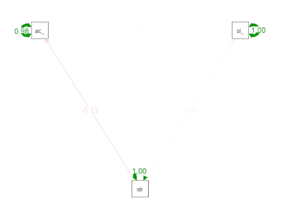
During this day, I will learn about the use of SEM in Psychology (Cognitive and Behavioral Research). The example is investigating the relationship between stress, self-esteem, and academic performance. For this example, the model is that stress negatively affects self-esteem, which in turn impacts academic performance. SEM helps to model the direct effect of stress on performance, as well as the indirect effect via self-esteem. A hypothetical dataset will be used.

Initially, lavaan and semPlot packages are loaded, and a hypothetical dataset is developed, using the following lines of codes:

 

library(lavaan)

library(semPlot)

 

# Create a sample dataset

set.seed(123) # For reproducibility

n <- 100 # Number of participants

 

data <- data.frame(

  stress = rnorm(n, mean = 50, sd = 10),          # Stress scores

  self_esteem = rnorm(n, mean = 70, sd = 10),     # Self-esteem scores

  academic_performance = rnorm(n, mean = 75, sd = 10) # Academic performance scores

)

 

# Check the dataset

head(data)

 

Then, we define the relationships between the variables. For instance, stress directly affects self-esteem, self-esteem directly affects academic performance, and stress indirectly affects academic performance through self-esteem. These relationships can be written as follows:

 

# Define the SEM model

model <- '

  # Direct effects

  self_esteem ~ stress

  academic_performance ~ self_esteem

 

  # Indirect effect via self_esteem

  academic_performance ~ stress

'

Then, the lavaan function is used to fit the model, using the following lines of codes:

# Fit the SEM model

fit <- sem(model, data = data)

 

# Check the summary of the model

summary(fit, fit.measures = TRUE, standardized = TRUE)

 

The summary provides important information, including path coefficients, standard errors, p-values, and fit indices like RMSEA, CFI, and TLI.

 

Then, the results are interpreted using the summary(fit) function. For instance, Path Coefficients show the strength and direction of relationships between variables; Significance check the p-values to determine whether relationships are statistically significant; and Fit Indices show Good model fit is indicated by RMSEA < 0.06, CFI > 0.95, and TLI > 0.95.

 

Then, the model is visualized with semPlot package, using the following lines of codes:

 

# Plot the SEM model

semPaths(fit, what = "std",

         layout = "tree",

         edge.label.cex = 1.2,

         sizeMan = 6,

         sizeLat = 8)

 

The model can also be modified using the following:

# Define a new SEM model with mediation

mediation_model <- '

  # Mediation

  self_esteem ~ stress

  academic_performance ~ self_esteem

  academic_performance ~ stress

'

 

# Fit the new model

mediation_fit <- sem(mediation_model, data = data)

 

# Summary with fit measures

summary(mediation_fit, fit.measures = TRUE, standardized = TRUE)

 

# Visualize the mediation model

semPaths(mediation_fit, what = "std",

         layout = "circle",

         edge.label.cex = 1.2,

         sizeMan = 6,

         sizeLat = 8)

 

Source:
ChatGPT