Day 1: A challenge to learn basics of Structural Equation Modeling (SEM) using lavaan and semPlot packages in R

During the next 12 days, I will learn and repeat the basics of structural equation modeling (SEM) using lavaan and semPlot packages in R.

You can search my lavaan posts by typing: #UsmanZafarParacha_lavaan , and semPlot posts by typing: #UsmanZafarParacha_semPlot

============

During this day, I will learn about the use of SEM in Psychology (Cognitive and Behavioral Research). The example is investigating the relationship between stress, self-esteem, and academic performance. For this example, the model is that stress negatively affects self-esteem, which in turn impacts academic performance. SEM helps to model the direct effect of stress on performance, as well as the indirect effect via self-esteem. A hypothetical dataset will be used.

Initially, lavaan and semPlot packages are loaded, and a hypothetical dataset is developed, using the following lines of codes:

 

library(lavaan)

library(semPlot)

 

# Create a sample dataset

set.seed(123) # For reproducibility

n <- 100 # Number of participants

 

data <- data.frame(

  stress = rnorm(n, mean = 50, sd = 10),          # Stress scores

  self_esteem = rnorm(n, mean = 70, sd = 10),     # Self-esteem scores

  academic_performance = rnorm(n, mean = 75, sd = 10) # Academic performance scores

)

 

# Check the dataset

head(data)

 

Then, we define the relationships between the variables. For instance, stress directly affects self-esteem, self-esteem directly affects academic performance, and stress indirectly affects academic performance through self-esteem. These relationships can be written as follows:

 

# Define the SEM model

model <- '

  # Direct effects

  self_esteem ~ stress

  academic_performance ~ self_esteem

 

  # Indirect effect via self_esteem

  academic_performance ~ stress

'

Then, the lavaan function is used to fit the model, using the following lines of codes:

# Fit the SEM model

fit <- sem(model, data = data)

 

# Check the summary of the model

summary(fit, fit.measures = TRUE, standardized = TRUE)

 

The summary provides important information, including path coefficients, standard errors, p-values, and fit indices like RMSEA, CFI, and TLI.

 

Then, the results are interpreted using the summary(fit) function. For instance, Path Coefficients show the strength and direction of relationships between variables; Significance check the p-values to determine whether relationships are statistically significant; and Fit Indices show Good model fit is indicated by RMSEA < 0.06, CFI > 0.95, and TLI > 0.95.

 

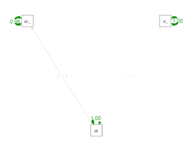
Then, the model is visualized with semPlot package, using the following lines of codes:

 

# Plot the SEM model

semPaths(fit, what = "std",

         layout = "tree",

         edge.label.cex = 1.2,

         sizeMan = 6,

         sizeLat = 8)

 

The model can also be modified using the following:

# Define a new SEM model with mediation

mediation_model <- '

  # Mediation

  self_esteem ~ stress

  academic_performance ~ self_esteem

  academic_performance ~ stress

'

 

# Fit the new model

mediation_fit <- sem(mediation_model, data = data)

 

# Summary with fit measures

summary(mediation_fit, fit.measures = TRUE, standardized = TRUE)

 

# Visualize the mediation model

semPaths(mediation_fit, what = "std",

         layout = "circle",

         edge.label.cex = 1.2,

         sizeMan = 6,

         sizeLat = 8)

 

Source:
ChatGPT